Beginner to Advanced IF Function in Excel-9 Examples

Among the logical functions in Excel, the IF function is the most commonly used. It is extremely rare for an Excel user, whether novice or advanced, to never use the IF function.

In a nutshell, the IF function returns custom values that correspond to multiple conditions. When the IF function is nested or embedded with other functions in Excel, its applications expand.

In this article, we will learn several ways to use the IF function with examples that will be useful for both beginners and advanced users of MS Excel.

Syntax of IF Function

=IF(logic, return1, return2)

Argument of IF Function

logic- logical expression or value to be evaluated

return1-value to return if the ‘’logic’’ is satisfied.

return2-value to return if the “logic” is not satisfied.

return1 and return2  can be text or any numerical value.

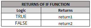
Return of IF Function

The IF function operates based on TRUE or FALSE returns from the logical argument. You can set the customized value to return based on the logical test’s TRUE or FALSE results.

According to the syntax of the IF function, the returns of the IF function are given below.

9 Examples of Basic to Advanced IF function in Excel

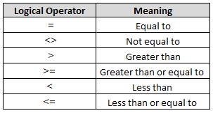
Before Jumping to examples you should know about the logical operators in Excel

Example #1: Simple Application of IF Function

Let’s try a simple example of the application of the IF function.

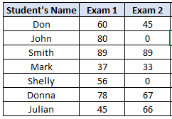
Assume you are given the following information: the student’s name and their English test scores.

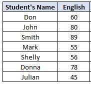
You want to write a formula to return if the obtained score is greater than 50 then “Passed”

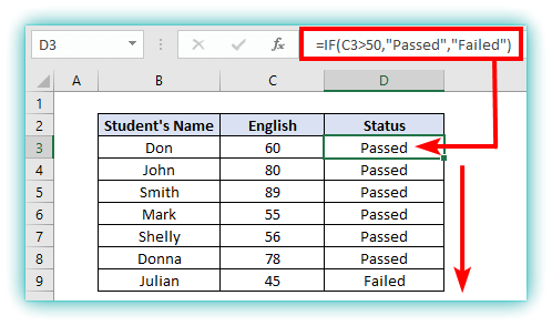
You can simply apply the IF formula as below.

=IF(C3>50,"Passed","Failed")

• Input the above formula in the output cell D3
• Press the Enter 
• AutoFill the resting cells in column D

Explanation:

• According to the syntax of the IF function, if C3>50 returns TRUE, then the IF function returns “Passed”. Otherwise, the IF function will return “Failed”.

See the formula evaluation for Don

=IF(C3>50,"Passed","Failed")

=IF(TRUE,"Passed","Failed")

=Passed

Example #2: Application of IF with Multiple Conditions

The first example’s data set is modified to include the obtained score in two new subjects: math and geography.

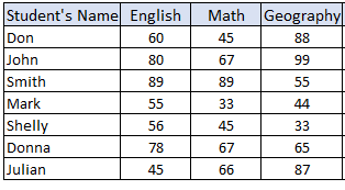
You want to know if the students scored higher than 50 in all three subjects.

We will use the AND function to combine three conditions for the three subjects.

The structured formula will be as below:

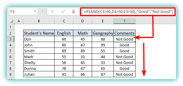
=IF(AND(C3>50,D3>50,E3>50),"Good","Not Good")

• Input the above formula in cell F3 and press Enter.
• Then Just AutoFill

Explanation: 

• The AND function will return TRUE if all three conditions inside the AND function are satisfied.
• If the AND function returns TRUE, then the IF function will return “Good”. Otherwise, the IF function will return “Not Good”.

Let’s see the formula evaluation for Don

=IF(AND(C3>50,D3>50,E3>50),"Good","Not Good")

=IF(AND(60>50,45>50,88>50),"Good","Not Good")

=IF(AND(TRUE,FALSE,TRUE),"Good","Not Good")

=IF(FALSE,"Good","Not Good")

=Not Good

Example #3: Application of Nested IF Function 

With reference to the previous example, you want to show results according to the following criteria:

The formula will be

=IF(C3>50,IF(D3>50,IF(E3>50,"Passed in all Exam","Failed in all Exam"),"Failed in Exam2"),"Failed in Exam1")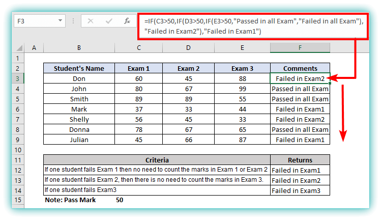

Explanation: 

• If condition C3>50 is satisfied, then the IF function will enter the nested second IF function and trigger the second IF function. Otherwise, the first IF function jumps to returning ‘’Failed in Exam1″
• Then, if condition D3>50 is satisfied, the IF function will trigger the third IF function. Otherwise, the second IF function jumps to returning “Failed in Exam 2.”
• Similarly, if condition E3>50 is satisfied, the third IF function returns “Passed in all Exams.” Otherwise, the third IF function jumps to returning “Failed in all Exams”

See the formula evaluation for Don

=IF(C3>50,IF(D3>50,IF(E3>50,"Passed in all Exam","Failed in all Exam"),"Failed in Exam2"),"Failed in Exam1")

=IF(60>50,IF(D3>50,IF(E3>50,"Passed in all Exam","Failed in all Exam"),"Failed in Exam2"),"Failed in Exam1")

=IF(TRUE,IF(D3>50,IF(E3>50,"Passed in all Exam","Failed in all Exam"),"Failed in Exam2"),"Failed in Exam1")

=IF(TRUE,IF(45>50,IF(E3>50,"Passed in all Exam","Failed in all Exam"),"Failed in Exam2"),"Failed in Exam1")

=IF(TRUE,IF(FALSE,IF(E3>50,"Passed in all Exam","Failed in all Exam"),"Failed in Exam2"),"Failed in Exam1")

=IF(TRUE,"Failed in Exam2","Failed in Exam1")

=Failed in Exam2

Example #4: Verify Array Conditions by IF Function

The IF function can be used to verify the array conditions. 

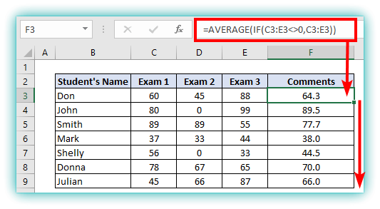
In this example, we want to determine the average score obtained across three exams.

But if any student gets a zero on any exam, then the corresponding cell should be avoided.

Let’s apply the following formula to solve this problem

=AVERAGE(IF(C3:E3<>0,C3:E3))

• Apply the above formula in the cell 
• After pressing Enter, AutoFill the remaining cells in the column 

Explanation: 

The IF function will check the values in the array that are not equal to 0. Then it returns the values that are not equal to zero.

Finally, the AVERAGE function calculates the average of the numbers returned by the IF function.

See the formula evaluation for John

=AVERAGE(IF(C4:E4<>0,C4:E4))

=AVERAGE(IF({TRUE,FALSE,TRUE},C4:E4))

=AVERAGE({80,FALSE,99})

=89.5

Example #5: Avoiding Errors by IF Function in Excel

When any number is divided by zero, Excel displays the #DIV/0! error.

In this example, we will avoid the #DIV/0! error by using the IF function with the help of the ISERROR function.

In the data set below, some students obtained zero in some subjects.

Let’s divide the score obtained in Exam1 by Exam 2 using the following formula

=IF(ISERROR(C3/D3),"Can't divide by Zero",C3/D3)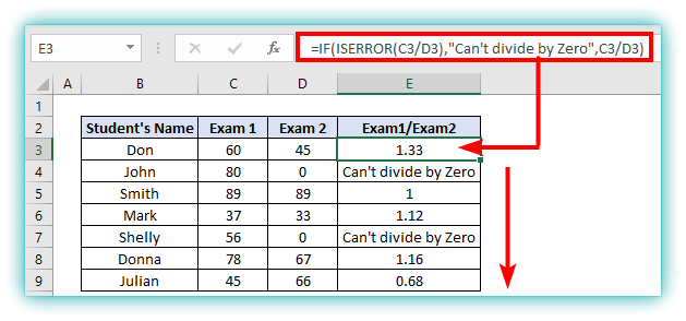

Explanation:

• The ISERROR function catches the errors in Excel. The ISERROR function returns TRUE when any error is displayed in the output cell.
• When the first logic, ISERROR(C3/D3), is TRUE, the IF function returns “Can’t divide by zero” in the output cell, according to the syntax of the IF function.

Let’s see the formula evaluation for John

=IF(ISERROR(C4/D4),"Can't divide by Zero",C4/D4)

=IF(TRUE,"Can't divide by Zero",C4/D4)

= Can't divide by Zero

You can rewrite the formula in the simplest version below

=IF(D3=0,"Can't divide by Zero",C3/D3)

You will get the same result, but in terms of processing speed, the ISERROR function is faster and more commonly used by professionals.

Example #6: Finding Blank Cell by IF Function in Excel

In the data given below, if any student is absent from the exam then the cell is kept blank

You want to show a user-friendly message that corresponds to whether the student was present or absent.

Apply the following formula to achieve the desired output:

=IF(ISBLANK(C3),"Not Present","Present")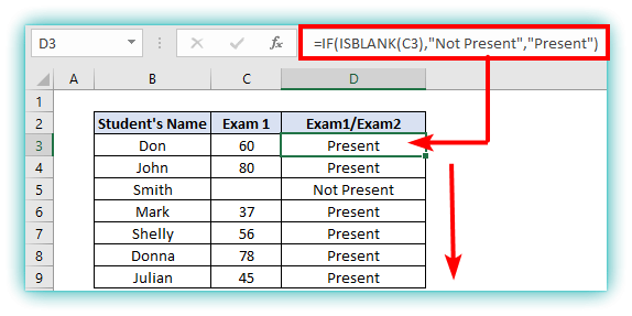

Explanation:

• The ISBLANK function returns TRUE if the cell given in the argument is really empty.
• Then the IF function returns “Not Present” when the ISBLANK function returns TRUE; otherwise, the IF function returns “Present”.

See the formula evaluation for Smith

=IF(ISBLANK(C5),"Not Present","Present")

=IF(TRUE,"Not Present","Present")

=Not Present

Example #7: Application of IF function to Verify Multiple Boolean Logic

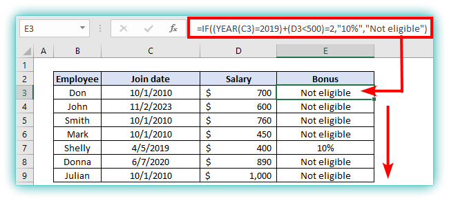
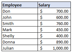
In the data table provided below, the employee name, join date, and salary are provided.

You want to give a 10% bonus to the employees whose joining year is 2019 and whose salary is less than $500.

We’ll use the YEAR function to see if the joining year is 2019 or not.

• Apply the following formula in the output cell E3

=IF((YEAR(C3)=2019)+(D3<500)=2,"10%","Not eligible")

• Press the Enter key on your keyboard
• Then AutoFill the remaining cell on the column E

Explanation:

• We know that the equivalent value of the Boolean return TRUE or FALSE is 1 or 0, respectively.
• YEAR(C3)=2019 returns TRUE or 1 when the year match with 2019
• Similarly, when condition D3<500 is satisfied, it returns TRUE or 1.
• (YEAR(C3)=2019)+(D3<500)=2 returns TRUE if both conditions are TRUE. In other words, TRUE is returned when 1+1 = 2, which satisfies the condition (YEAR(C3)=2019)+(D3<500)=2.
• Then the IF function returns “10%” if the first statement, (YEAR(C3)=2019)+(D3<500)=2 returns TRUE. Otherwise, the IF function returns “Not eligible”

Let’s see the formula evaluation for Shelly

=IF((YEAR(C7)=2019)+(D7<500)=2,"10%","Not eligible")

=IF((TRUE,"10%","Not eligible")

=10%

Example #8: IF Function with VLOOKUP Function

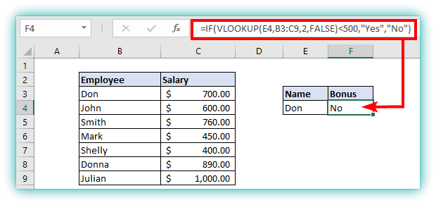
The IF function is widely used with the lookup functions in Excel. Suppose you want to give a bonus to the employees whose salaries are less than $500.

In this example, we will solve this problem by applying the IF function along with the VLOOKUP function.

• Input the following formula in the output cell F4

=IF(VLOOKUP(E4,B3:C9,2,FALSE)<500,"Yes","No")

• Hit the Enter key 

Explanation:

• VLOOKUP function will return the salary from the range B3:C9 corresponding to the entered value in cell E4
• Then VLOOKUP(E4,B3:C9,2,FALSE)<500 will return TRUE if the value returned by the formula VLOOKUP(E4,B3:C9,2,FALSE) is less than 500.
• If VLOOKUP(E4,B3:C9,2,FALSE)<500 returns TRUE, then the IF function will return “Yes”. otherwise, the IF function will return “No”

Let’s examine the formula explanation for Don,

=IF(VLOOKUP(E4,B3:C9,2,FALSE)<500,"Yes","No")

=IF(700<500,"Yes","No")

=IF(FALSE,"Yes","No")

=No

Example #9: IF Function with TEXT Function

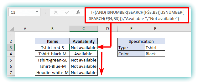
In this example, we will use the IF function to match the text value. For partial matching, we will use the ISNUMBER and SEARCH functions.

Suppose inventory data for items is given below.

You want to know the product availability for specific types and colors.

To solve this problem apply the following formula in the cell C3

=IF(AND(ISNUMBER(SEARCH(F$3,B3)),ISNUMBER(SEARCH(F$4,B3))),"Available ","Not available")

And then press the Enter button to AutoFill the residual cell in the column C.

Explanation:

• ISNUMBER(SEARCH(F$3,B3))  matches the input value in the cell F3 with the texts in cell B3
• Similarly ISNUMBER(SEARCH(F$4,B3)) matches the input value in the cell F4 with the texts in cell B3
• AND(ISNUMBER(SEARCH(F$3,B3)),ISNUMBER(SEARCH(F$4,B3)) returns TRUE only if the values in  cell F3 and F4 found in the cell B3
• If the AND function returns TRUE, then the IF function returns “Available “. Otherwise, the IF function returns “Not available“

See the formula evaluation below:

=IF(AND(ISNUMBER(SEARCH(F$3,B3)),ISNUMBER(SEARCH(F$4,B3))),"Available ","Not available")

=IF(AND(TRUE,FALSE),"Available ","Not available")

=IF(FALSE,"Available ","Not available")

=Not available

Things to Keep in Mind About the IF Function in Excel:

• The IF function does not care about the case. But the application of the EXACT function enables the IF function to be case-sensitive.
• Wildcards are not supported by the IF function. If applied with the SEARCH function, then the IF function can perform similarly.
• The IF function can be used to evaluate array conditions.
• When the given logical argument could be executed to return TRUE or FALSE, the #VALUE! error occurs.

Conclusion

We hope you have been elevated to an advanced level in applying the IF function in Excel. If this article, ’’ Beginner to Advanced IF Function in Excel ‘’ is really helpful, please provide feedback. Please comment below.