Shade Area Under Curve Excel

Suppose you have to shade the under-curve area in Excel for the equation given below

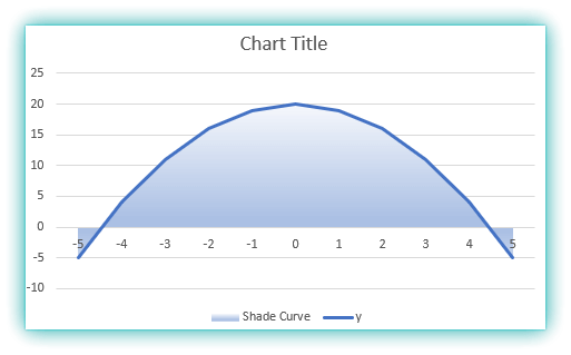
And you want to keep the line of the curve visible in a different color from the shaded area, as a sample output is given below:

Just follow the easy steps to get your desired result.

Step 01: To plot the curve, take some random value of x

Step 02: Write the curve equation in excel formula and enter it in cell C3 and AutoFill the remaining cells in column C to get the corresponding values of y. 

=-(B3^2)+20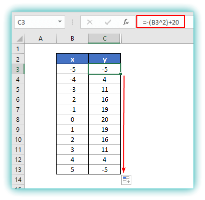

Step 03: Create a new column named Shade curve

Step 04: Insert the following formula in cell D3 and AutoFill the remaining cell in column D

=C3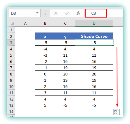

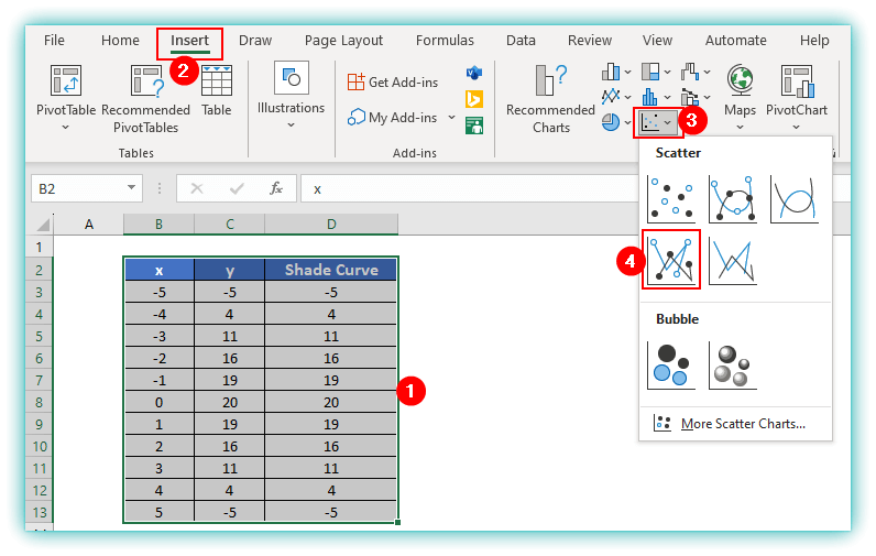
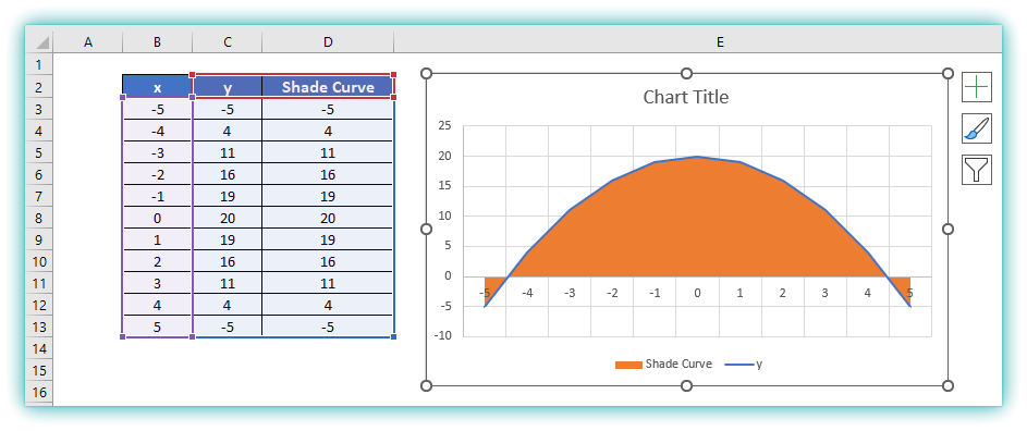
Step 05: Select the cell range B2:D13

Step 06: Go to the Insert tab

Step 07: From the charts section select the Scatter with Straight Line and Markers chart

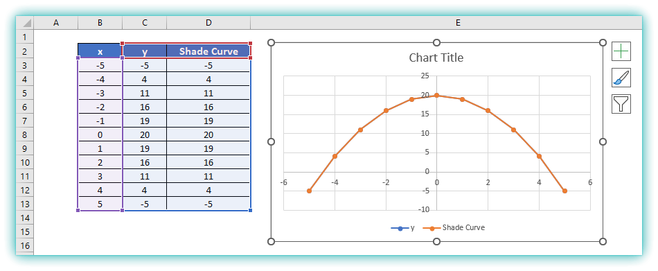
The output is

Step 08: Keeping the mouse pointer on the chart, Right click on the mouse

Step 09: A list of several options will appear, Click on the Change chart type

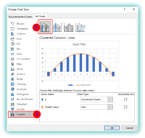
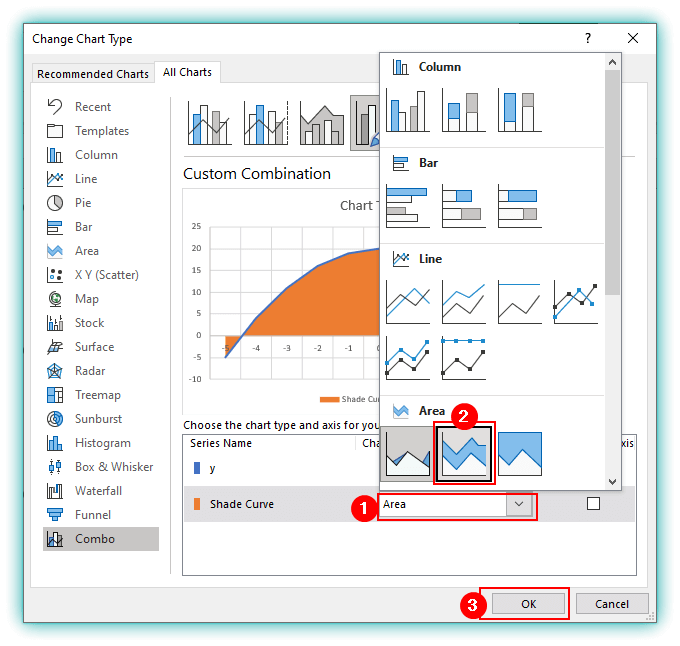
Step 10: A window named “Change Chart Type” will appear, click on the Combo

Step 11: Click on the Clustered Column Line

Step 12: Click on the Dropdown menu icon and Set the y series to Line 

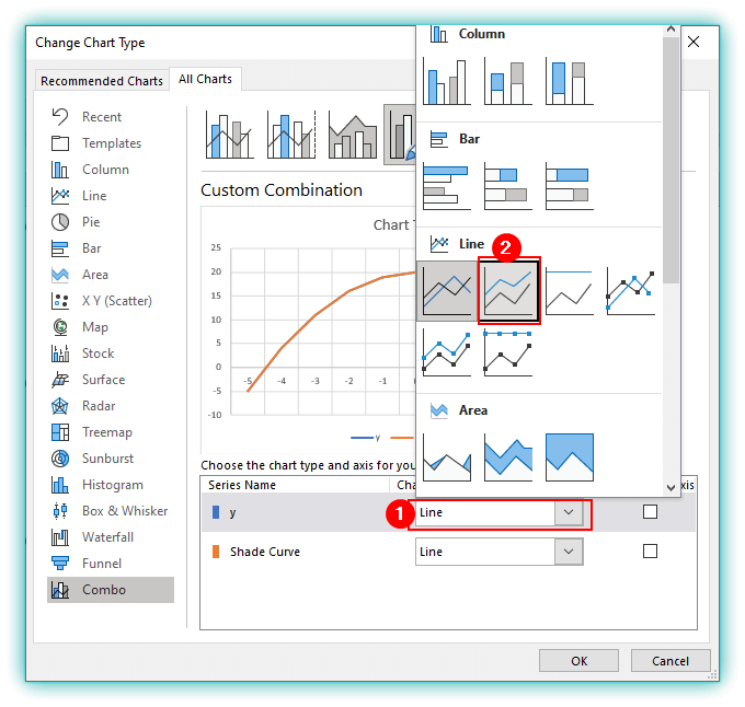
Step 13: Similarly, set the Shade area series to Area. Then Click on the OK

The result is

Customization of the curve:

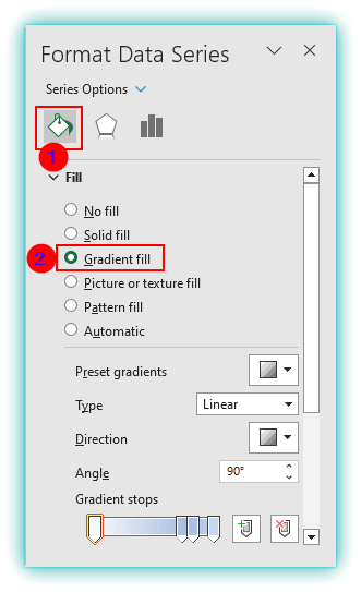
Step 01: Double-click on the curve area

Step 02: A window named “Format Data Series” will appear on the right side of the monitor. Click on the “Fill and Line” option. Here, you have plenty of options to customize the chart. Select Gradient fill or Pattern fill according to your preference.

The result is